Boston 범죄데이터 분석

1. 프로젝트 소개

boston 범죄데이터를 활용하여 범죄 유형을 예측하는 모델 구축,

머신러닝 모델의 하이퍼파라미터를 조정하여 모델의 예측 정확도를 향상시킴

 

 - 기술 스택

• 프로그래밍 언어: Python
• 라이브러리: Scikit-Learn, Matplotlib, Seaborn
• 모델링 기법: 랜덤 포레스트, 그래디언트 부스팅

2. 프로젝트 상세 설명

1. 데이터 로드 및 전처리

• 데이터의 기본 구조를 파악하고 결측치를 처리하여, 모델 학습에 적합한 형태로 데이터를 전처리
  
  

코드

from sklearn.preprocessing import LabelEncoder
from sklearn.model_selection import train_test_split

# 결측치 처리
New_DF['REPORTING_AREA'] = pd.to_numeric(New_DF['REPORTING_AREA'], errors='coerce')  # 숫자로 변환, 실패시 NaN으로 처리
New_DF = New_DF.dropna()  

x = New_DF[['DISTRICT', 'REPORTING_AREA', 'YEAR', 'MONTH', 'HOUR','Lat','Long',]]  # DISTRICT는 인코딩, 나머지는 그대로
y = New_DF['OFFENSE_CODE_GROUP']  

# 범주형 변수 인코딩 (DISTRICT만 원핫인코딩)
x_encoded = pd.get_dummies(x, columns=['DISTRICT'])

# y에서 상위 3개의 OFFENSE_CODE_GROUP만 필터링
top_offenses = y.value_counts().head(3).index
filtered_df = New_DF[New_DF['OFFENSE_CODE_GROUP'].isin(top_offenses)]

# 필터링된 데이터에서 X, Y 재설정
x_filtered = filtered_df[['DISTRICT', 'REPORTING_AREA', 'YEAR', 'MONTH', 'HOUR','Lat','Long']]
x_filtered_encoded = pd.get_dummies(x_filtered, columns=['DISTRICT'])
y_filtered = filtered_df['OFFENSE_CODE_GROUP']

# y에 대해 라벨 인코딩
label_encoder = LabelEncoder()
y_encoded = label_encoder.fit_transform(y_filtered)

# 데이터 분할 (훈련 데이터와 테스트 데이터)
x_train, x_test, y_train, y_test = train_test_split(x_filtered_encoded, y_encoded, test_size=0.2, random_state=42)

 

2. 하이퍼파라미터 설정 및 조정

• 모델의 성능에 영향을 미칠 수 있는 주요 하이퍼파라미터를 선정하여, 각각의 값에 따른 모델 성능을 비교.
• n_estimators: 트리의 개수를 의미하며, n_estimators 값에 따라 모델의 예측 성능이 어떻게 변하는지 분석.
• learning_rate: 학습률을 조정하여 학습 속도와 정확도 간의 균형을 맞추고자 함.
• max_depth: 트리의 최대 깊이를 설정하여 과적합(overfitting)을 방지.

코드

from sklearn.tree import DecisionTreeClassifier
from sklearn.ensemble import AdaBoostClassifier
import numpy as np
from sklearn.metrics import accuracy_score
from sklearn.metrics import f1_score

# 변수 초기화
best_accuracy = 0
best_n_estimators = None
best_learning_rate = None

# 하이퍼파라미터 설정
n_estimators_list = [10, 50, 100, 200]
learning_rate_list = [0.01, 0.1, 0.5, 1.0]

# 정확도를 저장할 배열 생성
accuracy_matrix = np.zeros((len(n_estimators_list), len(learning_rate_list)))
f1_matrix = np.zeros((len(n_estimators_list), len(learning_rate_list)))

# 모델 학습 및 정확도 저장
for i, n_estimators in enumerate(n_estimators_list):
    for j, learning_rate in enumerate(learning_rate_list):

        tree = DecisionTreeClassifier(max_depth=1)
        model = AdaBoostClassifier(estimator=tree, n_estimators=n_estimators, learning_rate=learning_rate, random_state=42,algorithm='SAMME')
        model.fit(x_train, y_train)

        # 예측
        y_train_pred = model.predict(x_train)
        train_accuracy = accuracy_score(y_train, y_train_pred)
        y_test_pred = model.predict(x_test)
        test_accuracy = accuracy_score(y_test, y_test_pred)
        test_f1 = f1_score(y_test, y_test_pred, average='weighted')
        
        # 정확도 기록
        accuracy_matrix[i, j] = test_accuracy  # 테스트 정확도 저장
        f1_matrix[i, j] = test_f1

        # best
        if test_accuracy > best_accuracy:
            best_accuracy = test_accuracy
            best_f1_score = test_f1
            best_n_estimators = n_estimators
            best_learning_rate = learning_rate

        print(f"n_estimators: {n_estimators}, learning_rate: {learning_rate} -> train 정확도: {train_accuracy * 100:.2f}%, test 정확도: {test_accuracy * 100:.2f}%, test F1 스코어: {test_f1:.2f}")

print(f"best \nn_estimators: {best_n_estimators}, learning_rate: {best_learning_rate} -> test 정확도: {best_accuracy * 100:.2f}%, test F1 스코어: {best_f1_score:.2f}")

결과

코드

# max_depth 리스트 생성
max_depth_list = [3, 5, 7, 10, 12, 15]

train_accuracy_list = []
test_accuracy_list = []
train_f1_list = []
test_f1_list = []
best_test_accuracy = 0
best_f1_score = 0
best_max_depth = None

# max_depth에 따른 성능 테스트
for max_depth in max_depth_list:
    # 모델 설정
    tree = DecisionTreeClassifier(max_depth=max_depth)
    model = AdaBoostClassifier(estimator=tree, n_estimators=best_n_estimators, learning_rate=best_learning_rate, random_state=42, algorithm='SAMME')
    model.fit(x_train, y_train)
    
    # 예측
    y_train_pred = model.predict(x_train)
    train_accuracy = accuracy_score(y_train, y_train_pred)
    train_accuracy_list.append(train_accuracy)


    y_test_pred = model.predict(x_test)
    test_accuracy = accuracy_score(y_test, y_test_pred)
    test_f1 = f1_score(y_test, y_test_pred, average='weighted')
    test_accuracy_list.append(test_accuracy)
    test_f1_list.append(test_f1)

    # 가장 높은 테스트 정확도 및 F1 스코어 저장
    if test_accuracy > best_test_accuracy or (test_accuracy == best_test_accuracy and test_f1 > best_f1_score):
        best_test_accuracy = test_accuracy
        best_f1_score = test_f1
        best_max_depth = max_depth

    # 결과 출력 (train/test 정확도 및 F1 스코어)
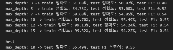
    print(f"max_depth: {max_depth} -> train 정확도: {train_accuracy * 100:.2f}%, test 정확도: {test_accuracy * 100:.2f}%, test F1: {test_f1:.2f}")

# 최적의 max_depth 출력
print(f"\nbest\nmax_depth: {best_max_depth} -> test 정확도: {best_test_accuracy * 100:.2f}%, test F1 스코어: {best_f1_score:.2f}")

결과

3. 모델 성능 시각화

• n_estimators와 learning_rate에 따른 정확도: n_estimators와 learning_rate 값에 따른 정확도 변화를 시각화하여, 하이퍼파라미터 조정이 모델에 미치는 영향을 파악
• Train/Test 정확도 비교: max_depth에 따른 학습 데이터와 테스트 데이터의 정확도를 비교하여, 모델이 과적합 또는 과소적합되는지 확인
• 히트맵: n_estimators와 learning_rate 조합에 따른 정확도를 히트맵으로 표현하여, 최적의 하이퍼파라미터 조합을 찾음

코드

import matplotlib.pyplot as plt
import seaborn as sns

fig, axs = plt.subplots(2, 2, figsize=(14, 10))

# n_estimators vs Accuracy by learning_rate
for j, learning_rate in enumerate(learning_rate_list):
    axs[0, 0].plot(n_estimators_list, accuracy_matrix[:, j], marker='o', label=f'Learning Rate = {learning_rate}')
axs[0, 0].set_title('n_estimators vs Accuracy by learning_rate')
axs[0, 0].set_xlabel('Number of Estimators')
axs[0, 0].set_ylabel('Accuracy')
axs[0, 0].legend(title='Learning Rates')
axs[0, 0].grid(True)

# Learning Rate vs Accuracy by n_estimators
for i, n_estimators in enumerate(n_estimators_list):
    axs[0, 1].plot(learning_rate_list, accuracy_matrix[i, :], marker='x', label=f'n_estimators = {n_estimators}')
axs[0, 1].set_title('Learning Rate vs Accuracy by n_estimators')
axs[0, 1].set_xlabel('Learning Rate')
axs[0, 1].set_ylabel('Accuracy')
axs[0, 1].legend(title='n_estimators')
axs[0, 1].grid(True)

# max_depth vs Accuracy (Train/Test 비교)
axs[1, 0].plot(max_depth_list, train_accuracy_list, marker='o', label='Train Accuracy')
axs[1, 0].plot(max_depth_list, test_accuracy_list, marker='x', label='Test Accuracy')
axs[1, 0].set_title('max_depth vs Accuracy (Train/Test)')
axs[1, 0].set_xlabel('max_depth')
axs[1, 0].set_ylabel('Accuracy')
axs[1, 0].legend()
axs[1, 0].grid(True)

#  히트맵 (n_estimators vs learning_rate에 따른 정확도)
sns.heatmap(accuracy_matrix, annot=True, cmap='coolwarm', xticklabels=learning_rate_list, yticklabels=n_estimators_list, ax=axs[1, 1])
axs[1, 1].set_title('Heatmap of Accuracy by n_estimators and learning_rate')
axs[1, 1].set_xlabel('Learning Rate')
axs[1, 1].set_ylabel('Number of Estimators')

# 그래프 간 여백 조정 및 시각화
plt.tight_layout()
plt.show()

결과

프로젝트 성과

• 하이퍼파라미터 튜닝 전 모델의 기본 정확도는 약 45%였으나, 최적의 하이퍼파라미터 조합을 통해 최종 정확도 55%를 달성했습니다.
• F1 Score는 0.35에서 0.55로 향상되었습니다.
• 하이퍼파라미터 조정으로 인해 과적합(overfitting)을 방지하고, 모델이 일반화된 데이터에도 높은 성능을 보이도록 개선하였습니다.

Boston_crime.ipynb

0.23MB